2.2. Chemical Space Exploration with Molecular Morphing by Example
Table of Contents
In the previous tutorial, we introduced some of the low level Molpher-lib features that enable its user to modify molecular structures in a randomized manner. In this part of the usage tutorial, we focus on high level features that handle chemical space exploration on larger scale by iterative application of chemical operators.
The core data structure responsible for building and maintaining suggested chemical space paths is the exploration tree. The exploration tree contains all generated morphs and is rooted at the source molecule and is grown by iteratively applying chemical operators first on the source molecule, then on its descendants and so on. This way multiple chemical space paths can be created and evaluated.
As the paths are generated, the compounds on them can be characterized by the value of an objective function. This function should somehow formalize the relationship between a chemical structure and its fitness for the task at hand. Therefore, interesting paths can be prioritized over others. This way, the exploration tree can hopefully lead us towards interesting new compounds without having to enumerate all possible chemistry.
In the original Molpher algorithm, the objective function is
simply the structural distance between morphs and a target molecule.
This way Molpher is able to connect pairs of molecules by iteratively generating
morphs from the source and prioritizing those that are getting closer to the target.
As a result, the algorithm converges to the target structure and stops
once the target is identified among the generated morphs (Fig. 2.2). This
algorithm is called the classic algorithm and is
implemented in the molpher.algorithms.classic module.
See also
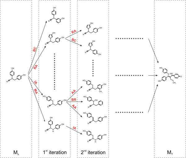
Fig. 2.2 Schematic depiction of the original algorithm published by Hoksza et al. 1.
New morphs are generated with chemical operators
applied to the source molecule (MS) until the target
molecule (MT) is found.
See also
Examples in this tutorial are included in a Jupyter Notebook
which can be downloaded here
viewed here. The example SDF can be found
here.
2.2.1. Creating an Exploration Tree and Setting Morphing Parameters
In Molpher-lib, the tree is implemented as the molpher.core.ExplorationTree class.
Following the captopril example from the previous tutorial,
the simplest way to generate an exploration tree instance is
to call the create() factory method:
1from molpher.core import ExplorationTree as ETree
2from molpher.core import MolpherMol
3
4captopril = MolpherMol("captopril.sdf")
5tree = ETree.create(source=captopril)
This code simply initializes the tree from the supplied MolpherMol instance.
At the moment the tree is pretty simple. It only contains the captopril structure as its
current leaves:
tree.leaves[0].asRDMol()
Output:
We can manipulate this tree and read data from it. Let’s start by printing out the source molecule:
print('Source: ', tree.params['source'])
Output:
Source: CC(CS)C(=O)N1CCCC1C(=O)O
The params member is a dictionary used to set and store morphing parameters:
print(tree.params)
Output:
{
    'source': 'CC(CS)C(=O)N1CCCC1C(=O)O',
    'target': None,
    'operators': (
        'OP_ADD_ATOM',
        'OP_REMOVE_ATOM',
        'OP_ADD_BOND',
        'OP_REMOVE_BOND',
        'OP_MUTATE_ATOM',
        'OP_INTERLAY_ATOM',
        'OP_BOND_REROUTE',
        'OP_BOND_CONTRACTION'
    ),
    'fingerprint': 'FP_MORGAN',
    'similarity': 'SC_TANIMOTO',
    'weight_min': 0.0,
    'weight_max': 100000.0,
    'accept_min': 50,
    'accept_max': 100,
    'far_produce': 80,
    'close_produce': 150,
    'far_close_threshold': 0.15,
    'max_morphs_total': 1500,
    'non_producing_survive': 5
}
As we can see there is quite a lot of parameters that we can set,
but most of these affect the exploration process only if
some parts of the library are used in the context of the tree, especially tree operations
which we will discuss later. The most important parameters
will be explained in this tutorial, but you can see the
documentation for the ExplorationData class
(especially Table 1.1) for a more detailed reference.
We can adjust the morphing parameters during runtime as we like.
All we need to overwrite the params attribute
of our tree instance with a new dictionary:
# change selected parameters using a dictionary
tree.params = {
    'non_producing_survive' : 2
    , 'weight_max' : 500.0
}
print(tree.params)
Output:
{
    'source': 'CC(CS)C(=O)N1CCCC1C(=O)O',
    'target': None,
    'operators': (
        'OP_ADD_ATOM',
        'OP_REMOVE_ATOM',
        'OP_ADD_BOND',
        'OP_REMOVE_BOND',
        'OP_MUTATE_ATOM',
        'OP_INTERLAY_ATOM',
        'OP_BOND_REROUTE',
        'OP_BOND_CONTRACTION'
    ),
    'fingerprint': 'FP_MORGAN',
    'similarity': 'SC_TANIMOTO',
    'weight_min': 0.0,
    'weight_max': 500.0,
    'accept_min': 50,
    'accept_max': 100,
    'far_produce': 80,
    'close_produce': 150,
    'far_close_threshold': 0.15,
    'max_morphs_total': 1500,
    'non_producing_survive': 2
}
Here we just tightened the constraints on molecular weight
for the morphs that we allow to be incorporated in the tree
(applied only if the FilterMorphsOper operation or filterMorphs method
are used with certain options) and we decreased the number of acceptable ‘non-producing’
morph generations to 2. Non-producing generations are
generations of morphs that has not improved in the objective function
(e.g. structural distance). See Table 1.1 for details.
One thing to note is that if we supply an incomplete set of parameters
(like in the example above), only the parameters specified in the
supplied dictionary will be changed. Parameters not mentioned in
this dictionary will remain the same as before the assignment.
Warning
Changing individual values in the params dictionary will have no effect.
You always need to store a dictionary instance in it. This is because the value
is regenerated every time the attribute is accessed to always reflect the current
set of parameters valid for the current instance.
See also
2.2.2. Morph Generation and Exploration Tree Extension
This part of the tutorial outlines the steps involved in one iteration of a possible exploration algorithm. We explain how to generate new morphs from the leaves of the tree, how they can be filtered and how the tree is extended by attaching the chosen morphs as the next generation of leaves. We also show how the unfavorable paths (or their parts) can later be removed from the growing tree.
2.2.2.1. Morph Generation and Manipulation
Previously, we showed how to initialize an exploration tree. Now that we have one, we can take a look at how to use it for chemical space exploration.
Let us generate a few morphs from the current leaves of the tree. Currently, the tree has just one leaf (our source molecule, captopril):
print(tree.leaves) # show the current leaves of the tree (only the source so far)
tree.leaves[0].asRDMol()
Output:
(<molpher.core.MolpherMol.MolpherMol at 0x7f37a8a6d930>,)

Since we already have the built-in operators available by default, we can generate new structures from this starting molecule like so:
1tree.generateMorphs()
2print(len(tree.candidates))
Output:
28
The generateMorphs() method tells
the tree to generate some morphs
from the current leaves for us. The number of generated morphs
will depend mostly on the far_produce, close_produce and far_close_threshold
parameters. However, it also depends on other factors. For example, some structures
might not be parsed correctly and, thus, might not make it to the final list.
Also, a different number of morphs can be generated each time the method is run. That si due to
the non-deterministic character of the morphing algorithm which chooses the morphing operators to
use and parts of the structure to modify randomly. Duplicate
molecules (based on the canonical smiles string) are also removed.
We can access the newly generated morphs from the candidates
member of the tree instance. It is a tuple of MolpherMol instances.
These instances can be used to read and manipulate the generated morphs or
the compounds currently present in the tree.
Attention
The molecules saved in the candidates attribute of the tree actually do not
belong to the tree just yet. See Tree Extension for more information on
how tree ownership is assigned to molecules.
2.2.2.2. Sorting and Filtering
The order of the newly generated molecules in the candidates list has a meaning
for the search algorithm. The higher the position of a morph in this list,
the bigger the probability that we will attach it to the tree as a new leaf
(see PROBABILITY for details). Therefore, by sorting this list according
to a given objective function, it is possible to push the algorithm
into convergence.
As of yet, the only way to sort the
generated morphs is by calling the sortMorphs()
method on the tree instance or using the SortMorphsOper operation
(see Tree Operations for more). This sorts the molecules in the order of increasing value
of the objective function. Right now, the objective function value used
by the sortMorphs operation is the value of the dist_to_target property
of the given MolpherMol instance. By default, the value
of this property indicates the structural distance of the morph in question
from the target molecule.
Since in our case we did not specify a target, the dist_to_target property will
be set to the same value for all molecules:
{x.dist_to_target for x in tree.candidates}
Output:
{1.7976931348623157e+308}
However, the dist_to_target property value can be changed to basically any float number.
If users have a custom objective function they want to use in the search,
it is possible to write their calculated value to this property and as long as lower value means
better fitness of the morph, it should still make sense to use this function
in the context of Molpher-lib and its data structures.
Note
This part of the interface (especially the naming convention) will likely change in the future since a more general approach is needed in order to make sorting more customizable.
Previously, we introduced the concept of morph collectors, which are special functions that can be used to intercept morphs as they are created. Setting the objective function value for each morph is a perfect use case for them:
1def sascore_as_obj(morph, operator):
2    morph.dist_to_target = morph.sascore
3
4tree.generateMorphs([sascore_as_obj])
5print(len(tree.candidates))
6{x.dist_to_target for x in tree.candidates}
Output (some results omitted):
28

[4.304767951403637,
 4.161464339486345,
 3.8871106534610247,
 ...
 4.336516757110866,
 4.187278867161213,
 3.8893996483733346]
This code is essentially the same as in Listing 2.3,
but this time we chose to add a custom morph collector
(the sascore_as_obj function),
which will set a molecule’s SAScore as the objective
function value for all generated morphs. Notice
that the generateMorphs() method takes a list of collectors
so it is possible to chain them together.
They are applied in the order of appearance in the list.
As you can see, the list of candidates is not sorted, yet.
We need to call the sortMorphs() method to do that:
1tree.sortMorphs()
2
3[
4    (x.smiles, x.dist_to_target)
5    for idx,x in enumerate(tree.candidates)
6]
Output (some results omitted):
[('CC(C)C(=O)N1CCCC1C(=O)O', 3.3191105796423788),
 ('CC(CO)C(=O)N1CCCC1C(=O)O', 3.6043596148886445),
 ('CNC(CS)C(=O)N1CCCC1C(=O)O', 3.7075484704945465),
...
 ('O=C(O)C1CCCN1C(=O)C(CS)CBr', 4.404706288979395),
 ('CC(CSI)C(=O)N1CCCC1C(=O)O', 4.412717102918789),
 ('O=C(O)C1CCCN1C(=O)C(CF)CS', 4.420781866555153)]
Therefore, now the list of candidates is sorted according to their synthetic accessibility (compounds that are easier to prepare in vitro should have lower scores).
Now, we need to choose the morphs that
will form the next generation.
The candidates_mask property of ExplorationTree
serves exactly this purpose. Each position in this list corresponds to
one molecule in candidates and indicates
whether this molecule should be considered when
attaching new leaves to the tree (True) or not (False).
Here is an example implementation of a very simple filtering procedure:
 1# print the current candidates mask (all positions are on by default)
 2print("Old mask:", tree.candidates_mask)
 3
 4# accept only the first ten morphs in the sorted list (those with the lowest distance to target)
 5new_mask = [True if idx < 10 else False for idx, x in enumerate(tree.candidates_mask)]
 6
 7# save the new mask to the tree
 8tree.candidates_mask = new_mask
 9
10# show results
11print("New mask:", tree.candidates_mask)
12print("Molecules that passed the filter:")
13[
14    (x.smiles, x.dist_to_target)
15    for idx,x in enumerate(tree.candidates)
16    if tree.candidates_mask[idx] # get molecules that passed the filter only
17]
Output:
Old mask: (True, True, True, True, True, True, True, True, True, True, True, True, True, True, True, True, True, True, True, True, True, True)
New mask: (True, True, True, True, True, True, True, True, True, True, False, False, False, False, False, False, False, False, False, False, False, False)
Molecules that passed the filter:

[('CC(C)C(=O)N1CCCC1C(=O)O', 3.3191105796423788),
 ('CCC(C)C(=O)N1CCCC1C(=O)O', 3.404002369297247),
 ('CSCCC(=O)N1CCCC1C(=O)O', 3.613205289055311),
 ('CC(CS)C(=O)N1CCCC1C(=O)O', 3.804751376555311),
 ('O=C(O)C1CCCN1C(=O)CCS', 3.8871106534610247),
 ('O=C(O)C1CCCN1C(=O)CCCS', 3.9220880467166013),
 ('CC(S)CC(=O)N1CCCC1C(=O)O', 3.9366697951036973),
 ('O=C(O)C1CCCN1C(=O)C1CSC1', 3.9784865729838823),
 ('CC(S)C(=O)N1CCCC1C(=O)O', 3.9938638051851627),
 ('CC(NCS)C(=O)N1CCCC1C(=O)O', 4.076862613435724)]
In Listing 2.6, candidates_mask member was changed by writing
a list or a tuple of new values into it. This way we were able to select only the first ten morphs
that have the best SAScore value.
Warning
The mask should only be set after the morphs are sorted. If the mask is set and the order of morphs is changed, the mask will stay the same and will have to be updated to follow the new order.
See also
The library implements a few built-in filters. You can use the
filterMorphs() method or FilterMorphsOper operation to invoke them.
See the method’s documentation for more information
on the available filtering options.
2.2.2.3. Tree Extension
When we have the morphs selected, we can call
the extend() method. This will connect them to their respective parents
in our tree and they will become a new set of leaves:
 1# get the number of generations before
 2print(tree.generation_count)
 3
 4tree.extend() # connect the accepted morphs to the tree as new leaves
 5
 6# get the number of generations after
 7print(tree.generation_count)
 8
 9# grab the new leaves as a list sorted according to their distance from target
10sorted(
11    [
12        (x.getSMILES(), x.getDistToTarget())
13        for x in tree.leaves
14    ], key=lambda item : item[1]
15)
Output:
WARNING: Candidate morph: CC(CS)C(=O)N1CCCC1C(=O)O already present in the tree. Skipping...
0
1

[('CC(C)C(=O)N1CCCC1C(=O)O', 3.3191105796423788),
 ('CCC(C)C(=O)N1CCCC1C(=O)O', 3.404002369297247),
 ('CSCCC(=O)N1CCCC1C(=O)O', 3.613205289055311),
 ('CSC(C)C(=O)N1CCCC1C(=O)O', 3.8501001628456333),
 ('O=C(O)C1CCCN1C(=O)CCS', 3.8871106534610247),
 ('CCC(CS)C(=O)N1CCCC1C(=O)O', 3.8893996483733346),
 ('CSCC(C)C(=O)N1CCCC1C(=O)O', 3.916140148729842),
 ('O=C(O)C1CCCN1C(=O)CCCS', 3.9220880467166013),
 ('CC(S)CC(=O)N1CCCC1C(=O)O', 3.9366697951036973)]
We can see that after extending the tree, the selected morphs (see Listing 2.6)
had become the new leaves and that the tree’s
morph generation counter (generation_count) was increased by one. We also
got a warning about one structure not being added to the tree. It is the structure
of captopril itself, which is already there. Thus, it is automatically skipped to prevent us from going
in circles.
If we want to, we can generate an image depicting the new leaves and the operators used to create them like so:
from rdkit.Chem.Draw import MolsToGridImage

def get_locked_atoms(mol):
    return [(idx, atm) for idx, atm in enumerate(mol.atoms) if atm.is_locked]

def show_mol_grid(mols):
    locked_atoms = [[y[0] for y in get_locked_atoms(x)] for x in mols]
    return MolsToGridImage(
        [x.asRDMol() for x in mols]
        , subImgSize=(250,200)
        , highlightAtomLists=locked_atoms
        , legends=[x.parent_operator for x in mols]
    )

show_mol_grid(tree.leaves)
Output:
Note that the generated morphs satisfy the locks placed on the signature -pril substructure in the original SDF file. Therefore, the tree is guaranteed to only contain structures that have this structural pattern. At this point, it is probably easy to envision an approach with iterative application of the commands above which would allow us to generate many possible structures of novel -pril compounds. This could prove useful while exploring the structure-activity relationship in the development of new ACE inhibitors, for example. Here is an example how a simple exploration algorithm for this purpose could look like:
class PenalizeKnown:

    def __init__(self, tree, penalty):
        self._tree = tree
        self._penalty = penalty

    def __call__(self, morph, operator):
        if self._tree.hasMol(morph):
            morph.dist_to_target += self._penalty

for iter_idx in range(1,10):
    tree.generateMorphs([sascore_as_obj, PenalizeKnown(tree, 10)])
    tree.sortMorphs()

    tree.candidates_mask = [
        True if idx < 50 and tree.candidates[idx].sascore < 6
        else False
        for idx, x in enumerate(tree.candidates_mask)
    ]

    tree.extend()
As in previous example (Listing 2.4), this code uses SAScore as the objective function, but this time we added one more collector to penalize morphs that we already attached to the tree. This way we can use a similar filtering procedure as before and run the code iteratively. In every iteration, we accept at most 50 structures which have synthetic accessibility score lower than 6. Running ten iterations like this gives us almost 500 new structures in a few seconds. If we chose to ran the algorithm for a few hours, we would get thousands of compounds like this for subsequent screening. At this point, it is probably obvious that we could add more collectors that could adjust the fitness of each morph further. For example, we could penalize morphs that have too many atoms, stereocenters or other unwanted structural features.
As the final example in this section, we add a target molecule to the tree and show how to use Molpher-lib for the task Molpher was originally designed for, that is to search for chemical space paths. We will choose another ACE inhibitor as our target, enalapril:
# set enalapril as target
tree.params = {
    'target' : MolpherMol("O=C(O)[CH]2N(C(=O)[CH](N[CH](C(=O)OCC)CCc1ccccc1)C)CCC2")
}
tree.params
Output:
{'source': 'CC(CS)C(=O)N1CCCC1C(=O)O',
 'target': 'CCOC(=O)C(CCC1=CC=CC=C1)NC(C)C(=O)N1CCCC1C(=O)O',
 'operators': ('OP_ADD_ATOM',
  'OP_REMOVE_ATOM',
  'OP_ADD_BOND',
  'OP_REMOVE_BOND',
  'OP_MUTATE_ATOM',
  'OP_INTERLAY_ATOM',
  'OP_BOND_REROUTE',
  'OP_BOND_CONTRACTION'),
 'fingerprint': 'FP_MORGAN',
 'similarity': 'SC_TANIMOTO',
 'weight_min': 0.0,
 'weight_max': 500.0,
 'accept_min': 50,
 'accept_max': 100,
 'far_produce': 80,
 'close_produce': 150,
 'far_close_threshold': 0.15,
 'max_morphs_total': 1500,
 'non_producing_survive': 2}
Now that we have a target, we can leverage the features Molpher-lib inherited from Molpher to find a chemical space path between captopril and enalapril:
 1class FindClosest:
 2
 3    def __init__(self):
 4        self.closest_mol = None
 5        self.closest_distance = None
 6
 7    def __call__(self, morph):
 8        if not self.closest_mol or self.closest_distance > morph.dist_to_target:
 9            self.closest_mol = morph
10            self.closest_distance = morph.dist_to_target
11
12closest_info = FindClosest()
13while not tree.path_found:
14    tree.generateMorphs()
15    tree.sortMorphs()
16    tree.filterMorphs()
17    tree.extend()
18    tree.prune()
19    tree.traverse(closest_info)
20    print('Generation #', tree.generation_count, sep='')
21    print('Molecules in tree:', tree.mol_count)
22    print(
23        'Closest molecule to target: {0} (Tanimoto distance: {1})'.format(
24            closest_info.closest_mol.getSMILES()
25            , closest_info.closest_distance
26        )
27    )
Output (some contents omitted):
Generation #11
Molecules in tree: 405
Closest molecule to target: CCCC(C)NC(C)C(=O)N1CCCC1C(=O)O (Tanimoto distance: 0.47457627118644063)
Generation #12
Molecules in tree: 481
Closest molecule to target: CCOC(C)NC(C)C(=O)N1CCCC1C(=O)O (Tanimoto distance: 0.4576271186440678)
Generation #13
Molecules in tree: 555
Closest molecule to target: CCOC(=O)C(C)NC(C)C(=O)N1CCCC1C(=O)O (Tanimoto distance: 0.375)
...
Generation #42
Molecules in tree: 365
Closest molecule to target: CCOC(=O)C(CCC1=CC=C1)NC(C)C(=O)N1CCCC1C(=O)O (Tanimoto distance: 0.09259259259259256)
Generation #43
Molecules in tree: 395
Closest molecule to target: CCOC(=O)C(CCC1=CC=C1)NC(C)C(=O)N1CCCC1C(=O)O (Tanimoto distance: 0.09259259259259256)
Generation #44
Molecules in tree: 424
Closest molecule to target: CCOC(=O)C(CCC1=CC=CC=C1)NC(C)C(=O)N1CCCC1C(=O)O (Tanimoto distance: 0.0)
Since we have a target structure defined, the software now
automatically calculates the distance of each morph from the target
and inserts that into the dist_to_target property
at the time of generation (call to generateMorphs()).
Therefore, we don’t need any customized collector in this instance. We also
chose to use the built-in filters (the filterMorphs() method)
to prioritize morphs in the candidates property. This filtering also
includes a synthetic accessibility filter like the one we used above
(only structures with SAScore higher than 6 are considered).
There are also a few features in this code that we haven’t studied in detail, yet.
For example, we used the traverse() method here to find out the closest
molecule to the target after finishing each iteration. Thanks to
this we can watch the algorithm converge to the target structure. We also used the
prune() method which is used to remove
branches in the tree that are not converging towards the target. This helps
to curb exponential growth of the tree. How this method works is
discussed in more detail later.
If we want to get a hold of the molecules on the path, we can easily do so:
1path = tree.fetchPathTo(tree.params['target'])
2
3print(len(path))
4show_mol_grid(path)
Output:
42
Note
We can see that what appeared to be especially challenging for the algorithm was the creation of the aromatic ring at the end. This is an issue often observed with the original algorithm implemented in Molpher. It usually doesn’t take a long time to converge to a structure which is very similar to the target, but more effort is needed to actually generate the target structure itself. Fortunately, Molpher-lib has at least some answer to that (see Bidirectional Algorithm).
2.2.2.4. Tree Pruning
We cannot possibly grow the tree into all directions without soon running out of memory or wasting computational time on a non-prospective part of chemical space. Thus, a strategy to keep the number of explored putative paths to a minimum is needed. This can be achieved by discarding parts of the paths that are not improving in the value of the objective function (distance from the target molecule in the simplest case).
We call a molecule that has not generated any morphs closer to the target than itself
a non-producing molecule and we can set
the number of generations to wait before removing its descendants
with the non_producing_survive parameter.
Tree pruning can be requested anytime by calling the prune() method. In our example, the method didn’t prune
any paths, because the non_producing_survive parameter is set to 2 generations in this particular instance.
See also
In addition to the non_producing_survive parameter, there is the max_morphs_total parameter,
which imposes a restriction on the maximum number of
descendants of one non-producing molecule. If the number of all historic descendants
reaches this threshold, the molecule is removed along with the current descendants.
2.2.3. Summary
This concludes the introduction of the main Molpher-lib building blocks. Hopefully, you found these examples useful and they helped to answer your questions about molecular morphing in general or the library itself. If not, feel free to use the issue tracker to ask questions or report bugs that you find. In the following sections, we describe more advanced topics such as custom chemical operators or tree serialization.