3. Exploration Algorithms Implementations¶

3.1. Classic (Original) Algorithm¶

This is the algorithm published with the Molpher program [1]. It is the most basic algorithm that can be implemented and a lot of fundamental concepts of Molpher-lib are based on it. The other algorithms presented in this part of the documentation are modifications or extensions of the original. It is, therefore, recommended to read this section before moving on to the following ones.

The classic algorithm uses a single tree rooted at the source molecule (M_S). Using predefined chemical operators, it generates a new generation of structures from the leaves of this tree at every iteration (see Fig. 3.1). The new list of candidates is then sorted (using the SortMorphsOper operation) in ascending order according to their structural distance from the target molecule (M_T). Finally, the new structures are filtered with the FilterMorphsOper operation and survivors are attached to their parents in the tree. This is repeated until the target molecule is generated and appended to the tree.

As the computation proceeds, some tree branches are also pruned (see PruneTreeOper). This is necessary to prevent exponential growth of the tree by removing paths that are not getting closer to the target molecule.

If you wish to know more about the steps involved in this algorithm, a detailed description can be found in [1].

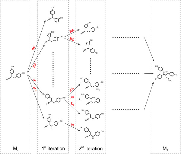
Fig. 3.1 Schematic depiction of the original algorithm published by Hoksza et al. [1]. New morphs are generated with the chemical operators until the target molecule is found.

The classic algorithm is available through the molpher.algorithms.classic package and can be used as follows:

 1
 2
 3
 4
 5
 6
 7
 8
 9
10
11
12
13
14
15
16
17
18
19
20
21
22
23
24
25
26
27
28
29
30
31

import os
import sys

from molpher.algorithms.classic.run import run
from molpher.algorithms.settings import Settings


def main(args):
    # our source and target molecules
    cocaine = 'CN1[C@H]2CC[C@@H]1[C@@H](C(=O)OC)[C@@H](OC(=O)c1ccccc1)C2'
    procaine = 'O=C(OCCN(CC)CC)c1ccc(N)cc1'

    # path to a directory where results will be stored (read from command line if possible)
    storage_dir = None
    if len(args) == 2:
        storage_dir = os.path.abspath(args[1])
    else:
        storage_dir = 'classic_data'

    # initialize the exploration settings
    settings = Settings(
        cocaine
        , procaine
        , storage_dir
        , max_threads=4
    )

    run(settings)

if __name__ == "__main__":
    exit(main(sys.argv))

The most essential ingredients in the example above are the run() function and the appropriate Settings class.

Every algorithm in the library has a run() function which calls the appropriate algorithm and saves the output of the computation. The run() function also supplies parameters to the tree and manages some ‘global’ aspects when a path is generated (such as the maximum number of threads to use).

The behaviour of run() is configured using a Settings class which is nothing more than a set of parameters wrapped into a class object. Some algorithms might define their own Settings classes with parameters specific to that algorithm. In this implementation, however, the most general Settings class is used.

In this instance, run() outputs a pickled list of SMILES strings which represents the resulting path into storage_dir.

3.2. Bidirectional Algorithm¶

The second algorithm included in the library is the bidirectional algorithm. The goal is the same as in the classic approach – to find a path from the source molecule to the target molecule. However, in this approach we use two trees (A and B) at once to get from M_S to M_T (see Fig. 3.2). One is set up to search for a path from M_S to M_T while the other searches in the opposite direction, that is from M_T to M_S.

After every complete iteration of the original algorithm in both trees (after the new structures are connected) the target molecule in each tree is replaced by the closest molecule to the current target from the opposite tree. This process is depicted in Fig. 3.2 where m_TA is found to be the closest molecule in tree B and, thus, becomes the new target of A. Similarly, molecule m_TB is the closest molecule to the current target of A and, therefore, becomes the new target of B. This causes that with each iteration the target of each tree becomes closer and closer. The algorithm ends when any of the two trees finds its target (the connecting_molecule). This structure is guaranteed to exist in both trees and is used to backtrack through them and generate the final path from M_S to M_T.

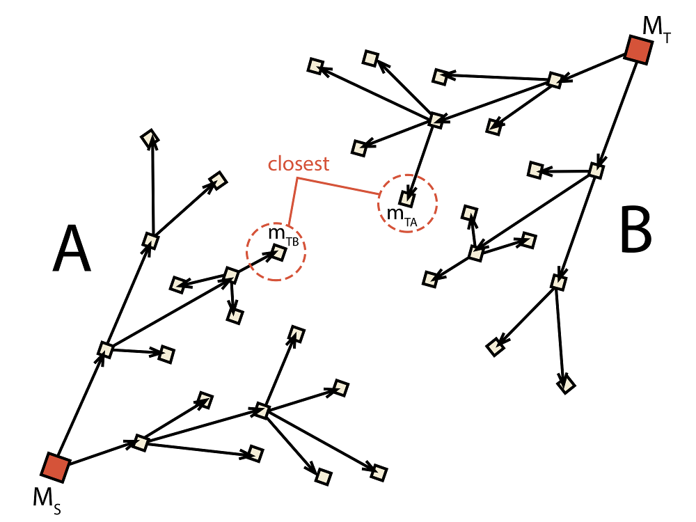
Fig. 3.2 Schematic depiction of the bidirectional algorithm. Two trees (A and B) are built at the same time with the target for each tree (m_TA for A and m_TB for B) being adjusted dynamically during runtime.

This algorithm should have some advantages over the classic one. The biggest is probably the fact that the space between M_S and M_T is explored in a more uniform way. The classic algorithm can often converge quickly to an area very close to M_T, but it usually takes a few more iterations before it finds the actual structure of M_T. This results in a disproportionate number of molecules on the path being highly similar to M_T. This is not the case for the bidirectional search where by the time the two trees get very close there is already a lot of similar molecules between them and it is much easier to find a connecting structure.

The bidirectional approach might also be able to converge quicker, because with each iteration the target gets closer and closer for each tree and this significantly reduces the search space.

The following script shows how this algorithm can be used to generate paths:

 1
 2
 3
 4
 5
 6
 7
 8
 9
10
11
12
13
14
15
16
17
18
19
20
21
22
23
24
25
26
27
28

import os

import sys

from molpher.algorithms.bidirectional.run import run
from molpher.algorithms.settings import Settings


def main(args):
    cocaine = 'CN1[C@H]2CC[C@@H]1[C@@H](C(=O)OC)[C@@H](OC(=O)c1ccccc1)C2'
    procaine = 'O=C(OCCN(CC)CC)c1ccc(N)cc1'
    storage_dir = None
    if len(args) == 2:
        storage_dir = os.path.abspath(args[1])
    else:
        storage_dir = 'bidirectional_data'

    settings = Settings(
        cocaine
        , procaine
        , storage_dir
        , max_threads=4
    )

    run(settings)

if __name__ == "__main__":
    exit(main(sys.argv))

The code above is almost identical to the example above (see Listing 3.1). It follows the same principles and the Settings class is also the same. The only difference is that the run method is imported from molpher.algorithms.bidirectional rather than molpher.algorithms.classic.

3.3. Anti-decoys Algorithm¶

The ‘anti-decoys algorithm’ is an extension of the bidirectional one and it tries to solve a problem that the algorithms above have in common. This problem is obvious when Molpher-lib is used to generate a focused library of compounds by pooling together structures from multiple exploration runs.

Even though the algorithms above are not deterministic, there is still a significant amount of overlap between the structures from multiple runs. This is due to the fact that in the cases above the algorithm is minimizing the distance between the source molecule and the target molecule which is important to actually be able to find a path, but is a problem when our aim is to generate a diverse library of structures because shorter paths will be preferred and, thus, contain highly similar compounds.

This unwanted behaviour is illustrated in Fig. 3.3 where the generated paths (dashed lines) between multiple compounds (shown in red) are seen to traverse a very limited area of chemical space (compounds marked with blue dots). However, it might still be possible to discover interesting structures if the algorithm took a little ‘detour’ and generated a path that is a bit longer, but contains some previously ‘unseen’ structures (shown as blue circles with question marks).

In the anti-decoys approach, this problem is eliminated by generating an ‘anti-fingerprint’. It is a 2D phramacophore fingerprint (implemented in RDKit) that contains information about all known and previously generated compounds. Because each bit in a pharmacophore fingerprint encodes information about geometric relationship of certain pharmacophore features in the structure, it is possible to cumulatively construct the anti-fingerprint by doing logical or over the fingerprints of previously discovered structures (see Fig. 3.3). Therefore, by minimizing the similarity to the anti-fingerprint and at the same time minimizing the structural distance from the target, the unexplored areas can be prioritized over those that were already sampled before.

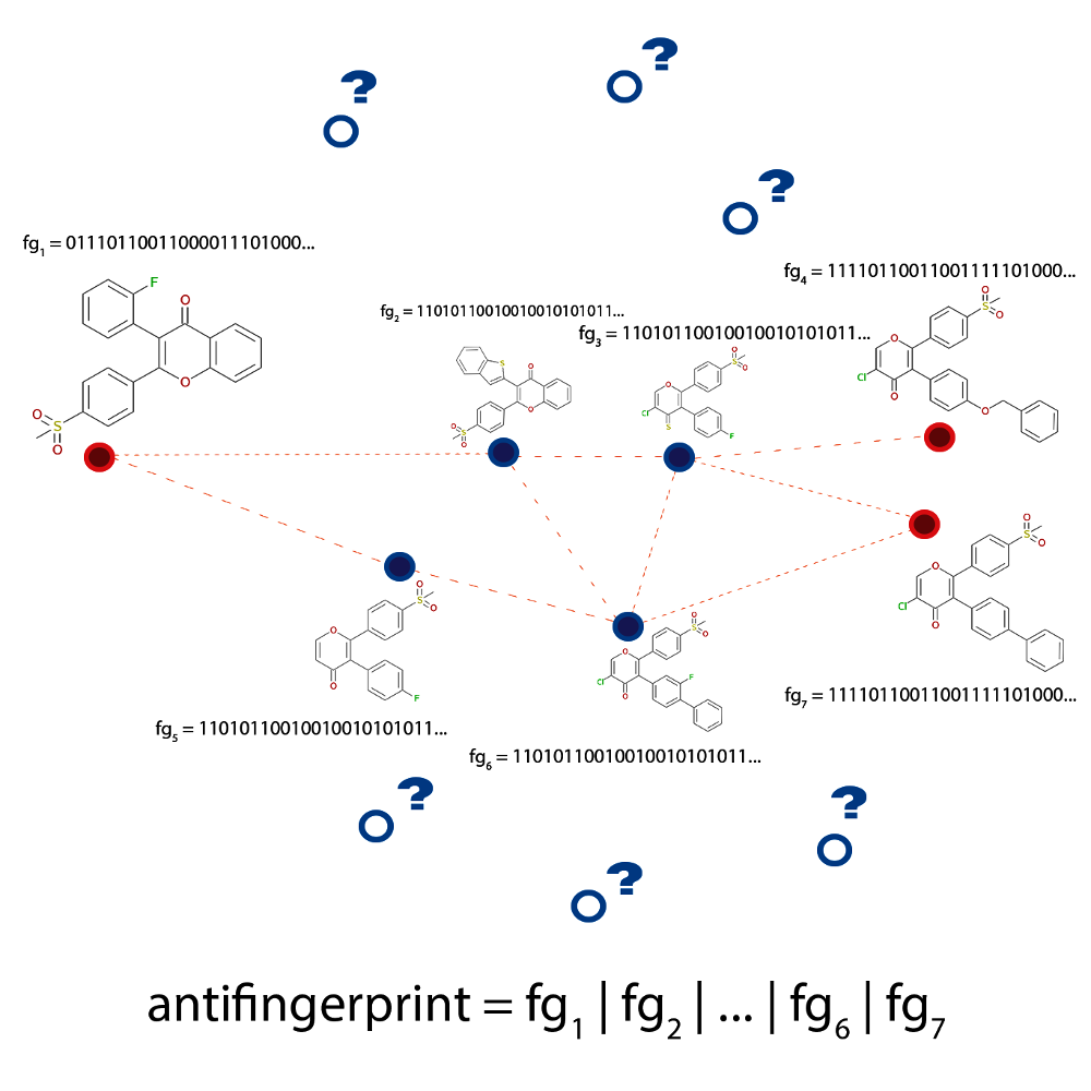
Fig. 3.3 Schematic depiction of the problem the anti-decoys algorithm tries to solve. The paths generated between active molecules (dashed lines connecting the red circles) are limited to an area of chemical space occupied by highly similar structures, the decoys (shown in blue). The algorithm analyses the decoys and uses this information to avoid them in future explorations using an anti-fingerprint that is computed as a logical or over all known fingerprints.

The antidecoys algorithm can be used as follows:

 1
 2
 3
 4
 5
 6
 7
 8
 9
10
11
12
13
14
15
16
17
18
19
20
21
22
23
24
25
26
27
28
29
30
31
32

import sys

from molpher.algorithms.antidecoys.run import run
from molpher.algorithms.antidecoys.settings import AntidecoysSettings

def main(args):
    cocaine = 'CN1[C@H]2CC[C@@H]1[C@@H](C(=O)OC)[C@@H](OC(=O)c1ccccc1)C2'
    procaine = 'O=C(OCCN(CC)CC)c1ccc(N)cc1'
    storage_dir = None
    if len(args) == 2:
        storage_dir = args[1]
    else:
        storage_dir = 'antidecoys_data'

    settings = AntidecoysSettings(
        source=cocaine
        , target=procaine
        , storage_dir=storage_dir
        , max_threads=4
        , common_bits_max_thrs = 0.75
        , min_accepted=500
        , antidecoys_max_iters=30
        , distance_thrs=0.3
    )

    run(
        settings
        , paths_count=50
    )

if __name__ == "__main__":
    exit(main(sys.argv))

This example is a little different from the ones before and there is a little bit more customization involved.

The antidecoys algorithm uses a customized settings class called AntidecoysSettings. In general, this class specifies important thresholds for the anti-fingerprint similarity and how strict the algorithm will be when filtering morphs. See the documentation of AntidecoysSettings to know more about this class and the additional parameters.

The run() function is also a bit different here. Because it is assumed that multiple paths will be generated, we also need to specify how many of them to find.

3.4. Summary¶

In this section, the implementations of various chemical space exploration algorithms were described. They are all based on the original algorithm implemented in Molpher, but the algorithms that can be implemented with the library do not have to be built on this basis. There are many ways to implement chemical space exploration using a library such as this one. For example, we are currently working on an implementation that will be independent of the target molecule and could be used to evolve compounds more freely with constraints imposed only by the user. Soon, we will also implement a way of preventing parts of the source molecule from being modified, which could be very useful in lead optimization. We are also planning to give users the option to define their own chemical operators, which will give an entirely new meaning to the generated paths. There are many ways in which this library could be useful in drug discovery, so if you have any suggestions or would like to actively participate on the project, it would be much appreciated. Make sure to visit the official GitHub repository for more information.